11.5ii: Heavy damping- $\gamma > 2\omega_{0}$

The motion is given by Equations 11.5.4 and 11.5.6 where, this time, $k_{1}$ and $k_{2}$ are each real and negative. For convenience, I am going to write $\lambda_{1}=-k_{1}$ and $\lambda_{2}=-k_{2}$. $\lambda_{1}$ are $\lambda_{2}$ both real and positive, with $\lambda_{2}$ > $\lambda_{1}$ given by

$$\lambda_{1}=\frac{1}{2}\gamma-\sqrt{(\frac{1}{2}\gamma)^{2}-\omega_{0}^{2}},\quad \lambda_{2}=\frac{1}{2}\gamma+\sqrt{(\frac{1}{2}\gamma)^{2}-\omega_{0}^{2}} \label{11.5.19}\tag{11.5.19}$$

The general solution for the displacement as a function of time is

$$x=Ae^{-\lambda_{1}t}+Be^{-\lambda_{2}t}. \label{11.5.20}\tag{11.5.20}$$

The speed is given by

$$\dot{x}=-A\lambda_{1}e^{-\lambda_{1}t}-B\lambda_{2}e^{-\lambda_{2}t}. \label{11.5.21}\tag{11.5.21}$$

The constants $A$ and $B$ depend on the initial conditions. Thus:

$$x_{0}=A+B \label{11.5.22}\tag{11.5.22}$$

and

$$(\dot{x})_{0}=-(A\lambda_{1}+B\lambda_{2}). \label{11.5.23}\tag{11.5.23}$$

From these, we obtain

$$A=\frac{(\dot{x})_{0}+\lambda_{2}x_{0}}{\lambda_{2}-\lambda_{1}},\qquad B=-[\frac{(\dot{x})_{0}+\lambda_{1}x_{0}}{\lambda_{2}-\lambda_{1}}]. \label{11.5.24}\tag{11.5.24}$$

Example $\PageIndex{1}$

$x_{0}\neq0,\quad(\dot{x})_{0}=0.$

$$x=\frac{x_{0}}{\lambda_{2}-\lambda_{1}}(\lambda_{2}e^{-\lambda_{1}t}-\lambda_{1}e^{-\lambda_{2}t}). \label{11.5.25}\tag{11.5.25}$$

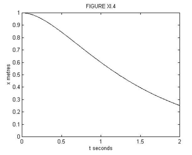
Figure XI.4 shows $x\quad:\quad t$ for $x_{0}$ = 1 m, $\lambda_{1}$ = 1 s^-1, $\lambda_{2}$ = 2 s^-1.

The displacement will fall to half of its initial value at a time given by putting $\frac{x}{x_{0}}=\frac{1}{2}$ in Equation $\ref{11.5.25}$. This will in general require a numerical solution. In our example, however, the equation reduces to $\frac{1}{2}=2e^{-t}-e^{-2t}$ and if we let $u=e^{-t}$, this becomes $u^{2}-2u+\frac{1}{2}=0$. The two solutions of this are $u=1.707107$ or $0.292893$. The first of these gives a negative t, so we want the second solution, which corresponds to $t= 1.228$ seconds.

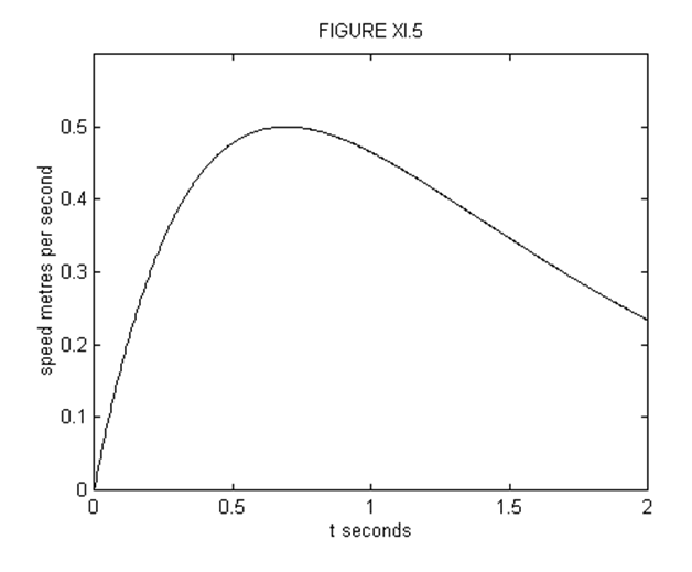
The velocity as a function of time is given by

$$\dot{x}=-\frac{\lambda_{1}\lambda_{2}x_{0}}{\lambda_{2}-\lambda_{1}}(e^{-\lambda_{1}t}-e^{\lambda_{2}t}). \label{11.5.26a}\tag{11.5.26a}$$

This is always negative. In figure XI.5, is shown the speed, which is $|\dot{x}|$ as a function of time, for our numerical example. Those who enjoy differentiating can show that the maximum speed is reached in a time $-\dot{x}$ and that the maximum speed is $\frac{\lambda_{1}\lambda_{2}x_{0}}{\lambda_{2}-\lambda_{1}}[(\frac{\lambda_{1}}{\lambda_{2}})^{\frac{\lambda_{2}}{\lambda_{2}-\lambda_{1}}}-(\frac{\lambda_{1}}{\lambda_{2}})^{\frac{\lambda_{1}}{\lambda_{2}-\lambda_{1}}}]$. (Are these dimensionally correct?) In our example, the maximum speed, reached at $t=\ln 2=0.6931$ seconds, is 0.5 m s^-1.

Example $\PageIndex{2}$

$x_{0}=0,\quad (\dot{x})_{0}=V(>0)$.

In this case it is easy to show that

$$x=\frac{V}{\lambda_{2}-\lambda_{1}}(e^{-\lambda_{1}t}-e^{-\lambda_{2}t}). \label{11.5.26b}\tag{11.5.26b}$$

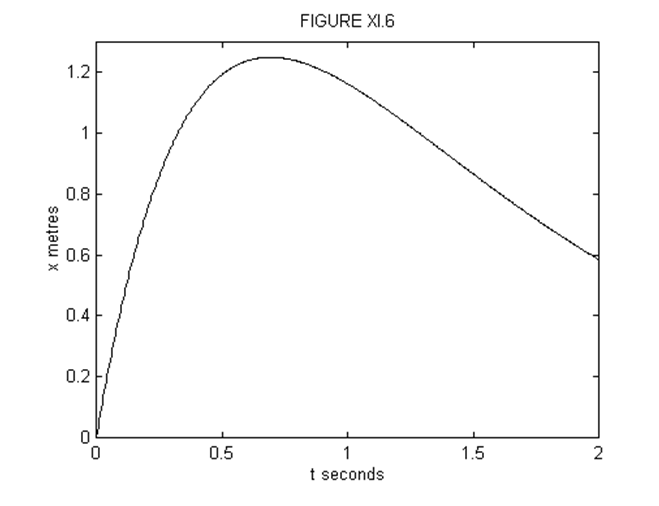
It is left as an exercise to show that $x$ reaches a maximum value of $\frac{V}{\lambda_{2}}(\frac{\lambda_{1}}{\lambda_{2}})^{\frac{\lambda_{1}}{\lambda_{2}-\lambda_{1}}}$ when $t=\frac{\ln(\frac{\lambda_{2}}{\lambda_{1}})}{\lambda_{2}-\lambda_{1}}$. Figure XI.6 illustrates Equation $\ref{11.5.26a}$ for $\lambda_{1}$ = 1 s^-1, $\lambda_{2}$ = 2 s^-1, $V$ = 5 m s^-1. The maximum displacement of 1.25 m is reached when $t = \ln 2 = 0.6831$ s. It is also left as an exercise to show that equation $\ref{11.5.26a}$ can be written

$$x=\frac{2Ve^{-\frac{1}{2}\lambda t}}{\lambda_{2}-\lambda_{1}}\sinh (\frac{1}{4}\gamma^{2}-\omega_{0}^{2}). \label{11.5.27}\tag{11.5.27}$$

Example $\PageIndex{3}$

$x_{0}\neq 0,\quad(\dot{x})_{0}=-V$.

This is the really exciting example, because the suspense-filled question is whether the particle will shoot past the origin at some finite time and then fall back to the origin; or whether it will merely tamely fall down asymptotically to the origin without ever crossing it. The tension will be almost unbearable as we find out. In fact, I cannot wait; I am going to plot $x$ versus $t$ in figure XI.7 for $\lambda_{1}$ = 1 s^-1, $\lambda_{2}$ = 2 s ^-1, $x_{0}$ = 1 m, and three different values of $V$, namely 1, 2 and 3 m s^-1.

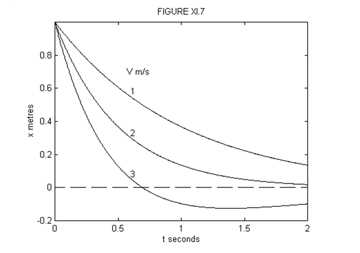
We see that if $V$ = 3 m s^-1 the particle overshoots the origin after about 0.7 seconds. If $V$ = 1 m s^-1, it does not look as though it will ever reach the origin. And if $V$ = 2 m s^-1, I'm not sure. Let's see what we can do. We can find out when it crosses the origin by putting $x$= 0 in Equation $\ref{11.5.20}$, where $A$ and $B$ are found from Equations $\ref{11.5.24}$ with $(\dot{x})_{0}=-V$. This gives, for the time when it crosses the origin,

$$t=\frac{1}{\lambda_{2}-\lambda_{1}}\ln(\frac{V-\lambda_{1}x_{0}}{V-\lambda_{2}x_{0}}). \label{11.5.28}\tag{11.5.28}$$

Since $\lambda_{2} > \lambda_{1}$, this implies that the particle will overshoot the origin if $V > \lambda_{2}x_{0}$, and this in turn implies that, for a given $V$, it will overshoot only if

$$\gamma < \frac{\frac{V^{2}}{x_{0}^{2}}+\omega_{0}^{2}}{\frac{V}{x_{0}}}. \label{11.5.29}\tag{11.5.29}$$

For our example, $\lambda_{2}x_{0}$= 2 m s^-1, so that it just fails to overshoot the origin if $V$= 2 m s^-1. For $V$ = 3 m s^-1, it crosses the origin at $t=\ln 2=0.6931$ s. In order to find out how far past the origin it goes, and when, we can do this just as in

I make it that it reaches its maximum negative displacement of -0.125 m at $t = \ln 4 = 1.386$ s.